Activation Functions For Deep Learning in Python
Activation function are used to bring non-linearities into decision boundary in the neural network. Reason for introducing non-linearities in data is to tackle real life scenario. Almost every data we deal in real life are nonlinear in nature. This is what makes neural network extremely powerful.
This article implements common activation functions which are used in deep learning algorithms in Python.
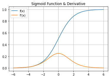
Sigmoid Function
One of the most commonly used activation function in deep learning is Sigmoid Function.
In mathematics, sigmoid is a function having a characteristic S-shaped curve or sigmoidal curve.
Output of sigmoid function is bounded between 0 and 1 which means we can use this as probability distribution.
Mathematical function for sigmoid is: $$ f(x) = \sigma(x) = \frac{1}{1+e^{-x}} $$
Derivative of sigmoid function is: $$ f'(x) = \sigma(x) ( 1 - \sigma(x) ) $$
Python Source Code: Sigmoidal Function
import numpy as np
from matplotlib import pyplot as plt

# Sigmoidal
def sig(x):
  return 1/(1+np.exp(-x))

# Sigmoidal derivative
def dsig(x):
  return sig(x) * (1- sig(x))

# Generating data to plot
x_data = np.linspace(-6,6,100)
y_data = sig(x_data)
dy_data = dsig(x_data)

# Plotting
plt.plot(x_data, y_data, x_data, dy_data)
plt.title('Sigmoid Function & Derivative')
plt.legend(['f(x)','f\'(x)'])
plt.grid()
plt.show()
Python Sigmoid Output
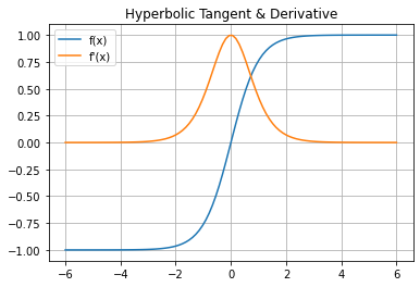
Tangent Hyperbolic Function
Another useful activation function is tangent hyperbolic.
Formula for Tangent Hyperbolic: $$ f(x) = \frac{e^{x} - e^{-x}}{e^{x} + e^{-x}} $$
Derivative for Tangent Hyperbolic is: $$ f'(x) = ( 1 - g(x)^{2} ) $$
Python Source Code: Tangent Hyperbolic
import numpy as np
from matplotlib import pyplot as plt

# Hyperbolic Tangent
def hyp(x):
  return (np.exp(x) - np.exp(-x))/(np.exp(x) + np.exp(-x))

# Hyperbolic derivative
def dhyp(x):
  return 1 - hyp(x) * hyp(x)

# Generating data to plot
x_data = np.linspace(-6,6,100)
y_data = hyp(x_data)
dy_data = dhyp(x_data)

# Plotting
plt.plot(x_data, y_data, x_data, dy_data)
plt.title('Hyperbolic Tangent & Derivative')
plt.legend(['f(x)','f\'(x)'])
plt.grid()
plt.show()
Python Tangent Hyperbolic Output
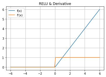
Rectified Linear Unit (RELU) Function
The rectified linear activation function (RELU) is a piecewise linear function that will output the input directly if it is positive, otherwise, it will output zero.
RELU has become the default activation function for different neural networks because a model that uses RELU is easier to train and it often achieves better performance.
Mathematical function for RELU is: $$ f(x) = max(0,x) $$
Derivative for RELU is: $$ f(x) = \begin{cases} \text{1, x>0} \\ \text{0, otherwise} \end{cases} $$
Python Souce Code: RELU
import numpy as np
from matplotlib import pyplot as plt

# Rectified Linear Unit
def relu(x):
  temp = [max(0,value) for value in x]
  return np.array(temp, dtype=float)
# Derivative for RELU
def drelu(x):
  temp = [1 if value>0 else 0 for value in x]
  return np.array(temp, dtype=float)

# Generating data to plot
x_data = np.linspace(-6,6,100)
y_data = relu(x_data)
dy_data = drelu(x_data)

# Plotting
plt.plot(x_data, y_data, x_data, dy_data)
plt.title('RELU & Derivative')
plt.legend(['f(x)','f\'(x)'])
plt.grid()
plt.show()
Python Output RELU